Regression analysis is a form of predictive modelling technique which investigates the relationship between a dependent (target) and independent variable (s) (predictor). This technique is used for forecasting, time series modelling and finding the causal effect relationship between the variables. For example, relationship between rash driving and number of road accidents by a driver is best studied through regression.
Linear Regression establishes a relationship between dependent variable (Y) and one or more independent variables (X) using a best fit straight line (also known as regression line). R provides comprehensive support for multiple linear regression.
Create a vector x from 1 to 100, added by normal distributed random value as noises
> x<-seq(1,100,by=1)+rnorm(100)
> x
Create y
> y<-x*15+rnorm(100,sd=50)+5
> y
Learn the Pearson Correlation between x and y
> cor.test(x,y)
Fit the linear regression model between x and y
> mydata<-data.frame(x,y)
> fit <- lm(y ~ x, data=mydata)
> summary(fit)
Show the model coefficient, squared R, and predicted y
> coefficients(fit)
> fitted(fit)
> summary(fit)$adj.r.squared
The linear model will be:
> formula<-paste0("y=",coefficients(fit)[2],"*x+",coefficients(fit)["(Intercept)"])
> formula
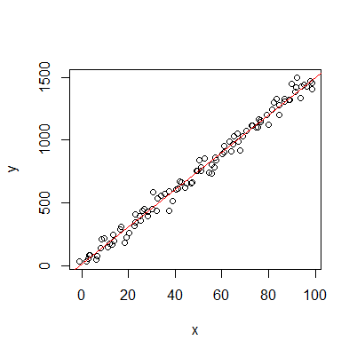
Plotting the linear regression
> plot(y~x)
> abline(fit, col="red")
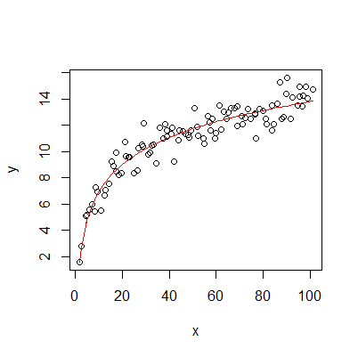
> x<-seq(1,100,by=1)+abs(rnorm(100))
> y<-log(x)*3+rnorm(100)
> mydata<-data.frame(x,y)
> fit<-lm(y~log(x),data=mydata)
> plot(y~x)
> lines(x,fitted(fit),col="red")
> The regression model will be:
> formula<-paste0("y=",coefficients(fit)[2],"*log(x)+",coefficients(fit)["(Intercept)"])
> formula
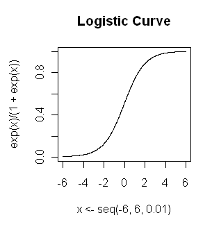
Logistic regression is used to find the probability of event=Success and event=Failure. We should use logistic regression when the dependent variable is binary (0/ 1, True/ False, Yes/ No) in nature. Here the value of Y ranges from 0 to 1 and it can represented by following equation.
odds= p/ (1-p) = probability of event occurrence / probability of not event occurrence
The natural log of odds is called the logit, or logit transformation, of p: logit(p) = loge(p/q)
Logistic regression is linear regression on the logit transform of y, where y is the proportion (or probability) of success at each value of x
y=p
ln(odds)=a+bx
ln(p/(1-p))=a+bx
ln(y/(1-y))=a+bx
exp(a+bx)=y/(1-y)
y=exp(a+bx)/[1+exp(a+bx)]
R makes it very easy to fit a logistic regression model. The function to be called is glm() and the fitting process is not so different from the one used in linear regression.
install.packages("MASS")
library("MASS")
data(menarche)
menarche[1:20,]
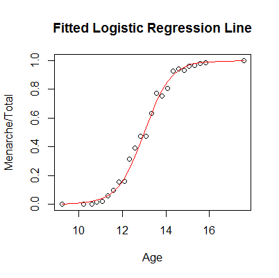
plot(Menarche/Total ~ Age, data=menarche)
The x is the age, and y is the probability of menarche. And the logistic fit can be done by (try to explain what is the the meaning of Menarche and Total-Menarche here):
glm.out = glm(cbind(Menarche, Total-Menarche) ~ Age, family=binomial(logit), data=menarche)
lines(menarche$Age, glm.out$fitted, type="l", col="red")
title(main="Fitted Logistic Regression Line")
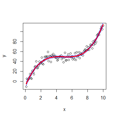
A regression equation is a polynomial regression equation if the power of independent variable is more than 1. The equation below represents a polynomial equation like: y=a*x^3+b*x^2+c*x+d
Generate the data
x<-seq(0.1,10,by=0.1)
y<-50+0.5*(x-5)^3+rnorm(100,sd=5)
plot(y~x)
Fit the model
fit <- lm(y ~ poly(x,3))
summary(fit)
Predicted values (fit value, lower and upper values of interval):
predicted.intervals <- predict(fit,data.frame(x),interval='confidence',level=0.95)
Add the fitted line on the plot
lines(x,predicted.intervals[,"fit"],col='red',lwd=3)
Add the interval lines on the plot
lines(x,predicted.intervals[,"lwr"],col='blue',lwd=1)
lines(x,predicted.intervals[,"upr"],col='blue',lwd=1)
Ridge Regression is a technique used when the data suffers from multicollinearity ( independent variables are highly correlated). By adding a degree of bias to the regression estimates, ridge regression reduces the standard errors.
Let a known matrix A(observed independent variables) and vector b (observed dependent variables). We wish to find a vector {x} that can build a linear regression: xA=b
However, if no x satisfies the equation or more than one x does, that leads to an over-fit or under-fit model.
Ordinary least squares seeks to minimize the sum of squared residuals, which can be compactly written as: ||betaA-b||^2
In order to give preference to a particular solution with desirable properties, a regularization term can be included in this minimization: ||betaA-b||^2+lambda*||beta||^2
Now try ridge regression in R
library(glmnet)
library(ISLR)
Hitters=na.omit(Hitters);with(Hitters,sum(is.na(Salary)))
x=model.matrix(Salary~.-1,data=Hitters)
y=Hitters$Salary
fit.ridge=glmnet(x,y,alpha=0) #alpha=0 means ridge-regression and alpha=1 means lasso regression
plot(fit.ridge,xvar="lambda",label=TRUE)
It makes a plot as a function of log of lambda, and is plotting the coefficients. glmnet develops a whole part of models on a grid of values of lambda (about 100 values of lambda).When log of lambda is 12, all the coefficients are essentially zero. Then as we relax lambda, the coefficients grow away from zero in a nice smooth way, and the sum of squares of the coefficients is getting bigger and bigger until we reach a point where lambda is effectively zero, and the coefficients are unregularized.
cv.ridge=cv.glmnet(x,y,alpha=0) #select the model
plot(cv.ridge) #show the mean-squared error for lambda values
cv.ridge #performance of models
cv.ridge$lambda.min #min lambda
cv.ridge$lambda.1se #lambda with standard error of the minimum
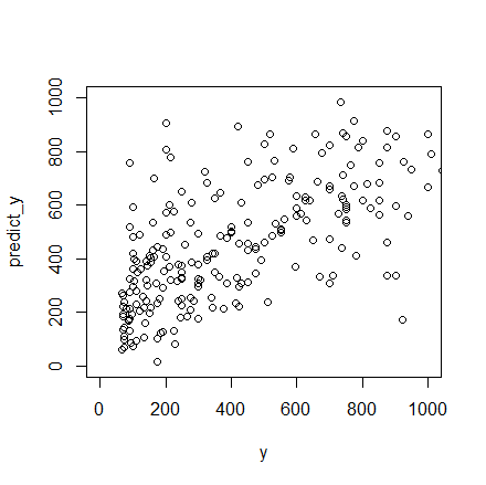
predict_y1<-predict(cv.ridge,x,s=cv.ridge$lambda.min) #predict y using the minimum lambda
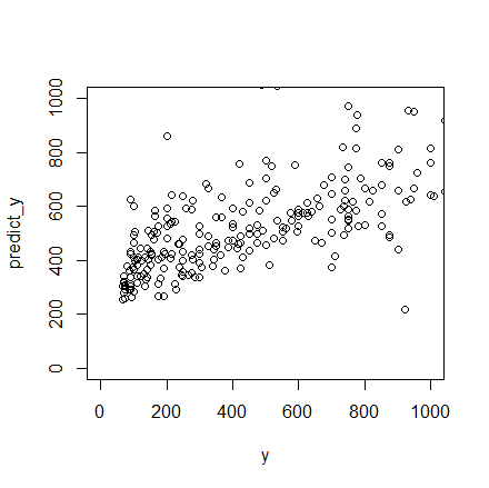
predict_y2<-predict(cv.ridge,x,s=cv.ridge$lambda.1se) #predict y using the 1se lambda
plot(y,predict_y1,xlim=c(0,1000),ylim=c(0,1000))
plot(y,predict_y2,xlim=c(0,1000),ylim=c(0,1000))
As part of the Bayesian framework, the Gaussian process specifies the prior distribution that describes the prior beliefs about the properties of the function being modeled. These beliefs are updated after taking into account observational data by means of a likelihood function that relates the prior beliefs to the observations. Taken together, the prior and likelihood lead to an updated distribution called the posterior distribution that is customarily used for predicting test cases. Interpretation of Ridge regression is available through Bayesian point estimation. In this setting the belief that beta should be small is coded into a prior distribution. As well, the form of the penalty term in Lasso regression can be interpreted as posterior mode estimates when the regression parameters have independent and identical Laplace (i.e., double-exponential) priors.
Similar to Ridge Regression, Lasso (Least Absolute Shrinkage and Selection Operator) also penalizes the absolute size of the regression coefficients. In addition, it is capable of reducing the variability and improving the accuracy of linear regression models. Lasso regression differs from ridge regression in a way that it uses absolute values in the penalty function, instead of squares. This leads to penalizing (or equivalently constraining the sum of the absolute values of the estimates) values which causes some of the parameter estimates to turn out exactly zero. Larger the penalty applied, further the estimates get shrunk towards absolute zero. This results to variable selection out of given n variables.
argmin ||betaA-b||^2+lambda*||beta||
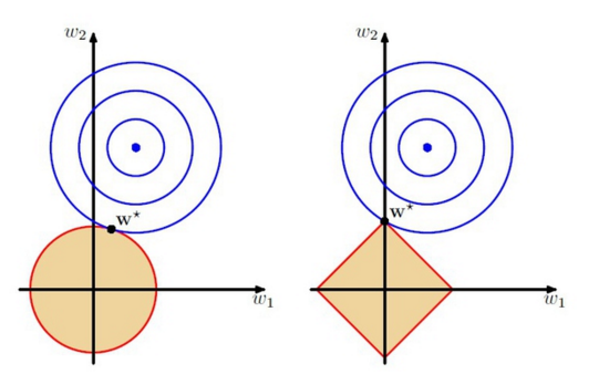
The w1 and w2 are the parameters, the orange regions are the regularization region. The w* is the predicted y, and its distance to the blue point is the error. The left figure is the ridge penalty and the right figure is the lasso penalty
Now try lasso regression in R
fit.lasso=glmnet(x,y,alpha=1)
plot(fit.lasso,xvar="lambda",label=TRUE)
cv.lasso=cv.glmnet(x,y) #cross validation to select model
plot(cv.lasso)
predict y
predict_y1<-predict(cv.ridge,x,s=cv.lasso$lambda.min) #predict y using the minimum lambda
predict_y2<-predict(cv.ridge,x,s=cv.lasso$lambda.1se) #predict y using the 1se lambda
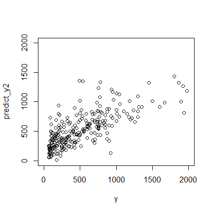
plot(y,predict_y1,xlim=c(0,2000),ylim=c(0,2000))
plot(y,predict_y2,xlim=c(0,2000),ylim=c(0,2000))

R |
R language |
plot |
|
barplot |
|
hist |
|
density |
|
boxplot |
|
heatmap |
tongyinbio@hku.hk bbru@hku.hk 13th-Feb 2017