Chip-seq tutorial

Introduction

One method to study transcription factor binding sites on a genome-wide level is via ChIP sequencing (ChIP-seq). ChIP-seq is a method that allows to identify genome-wide occupancy patterns of proteins of interest such as transcription factors, chromatin binding proteins, histones, DNA / RNA polymerases etc.

In this tutorial, we will use data come from ENCODE project (ENCSR000BOT). It is a ChIP-seq library prepared to analyze the REST transcription factor in human HepG2 cells. To shorten computational time required to run steps in this tutorial we scaled down dataset by keeping reads mapping to chromosome 20 only.

1. Prepare inputs

Change current directory

We will now make a subdirectory in your home directory to hold the files you will be creating and using in the course of this tutorial. To make a subdirectory called linuxstuff in your current working directory type

% cd ~

% mkdir chipseq

To see the directory you have just created, type ls

% cd chipseq

To see the directory you have jumped to, type pwd

Link reference genome and sequencing fq files to your working directory (chipseq).

% ln -s /home/source/chipseq/REST_HepG2/control.chr20.fq ./control.chr20.fq

% ln -s /home/source/chipseq/REST_HepG2/REST.chr20.fq ./REST.chr20.fq

% ln -s /home/reference/BroadInstitude_bundle/* ./

This option "-s" make "ln" provide a softlink from the raw data to your current directory

2. Sequence alignment

Use bwa mem to map input sequences in fq files to human genome

BWA is a software package for mapping low-divergent sequences against a large reference genome, such as the human genome. It consists of three algorithms: BWA-backtrack, BWA-SW and BWA-MEM. The first algorithm is designed for Illumina sequence reads up to 100bp, while the rest two for longer sequences ranged from 70bp to 1Mbp. BWA-MEM and BWA-SW share similar features such as long-read support and split alignment, but BWA-MEM, which is the latest, is generally recommended for high-quality queries as it is faster and more accurate. BWA-MEM also has better performance than BWA-backtrack for 70-100bp Illumina reads.

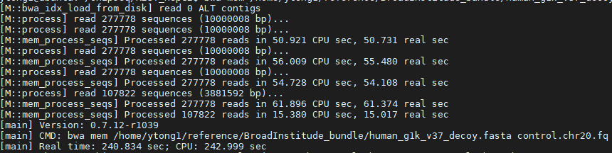
% bwa mem human_g1k_v37_decoy.fasta REST.chr20.fq > REST.chr20.sam

% bwa mem human_g1k_v37_decoy.fasta control.chr20.fq > control.chr20.sam

Question: what is the format and content of inputs and outputs

Tranform sam files to bams

% samtools view -S -b REST.chr20.sam > REST.chr20.bam

% samtools view -S -b control.chr20.sam > control.chr20.bam

Question: what is the difference between sam and bam format

OUTPUT: REST.chr20.bam

3. BAM file processing: sort, index

samtools sort REST.chr20.bam > REST.chr20.sorted.bam

samtools index REST.chr20.sorted.bam

Question: please repeat these steps for the control sample

OUTPUT: REST.chr20.sorted.bam

4. ChIP-seq peaks calling

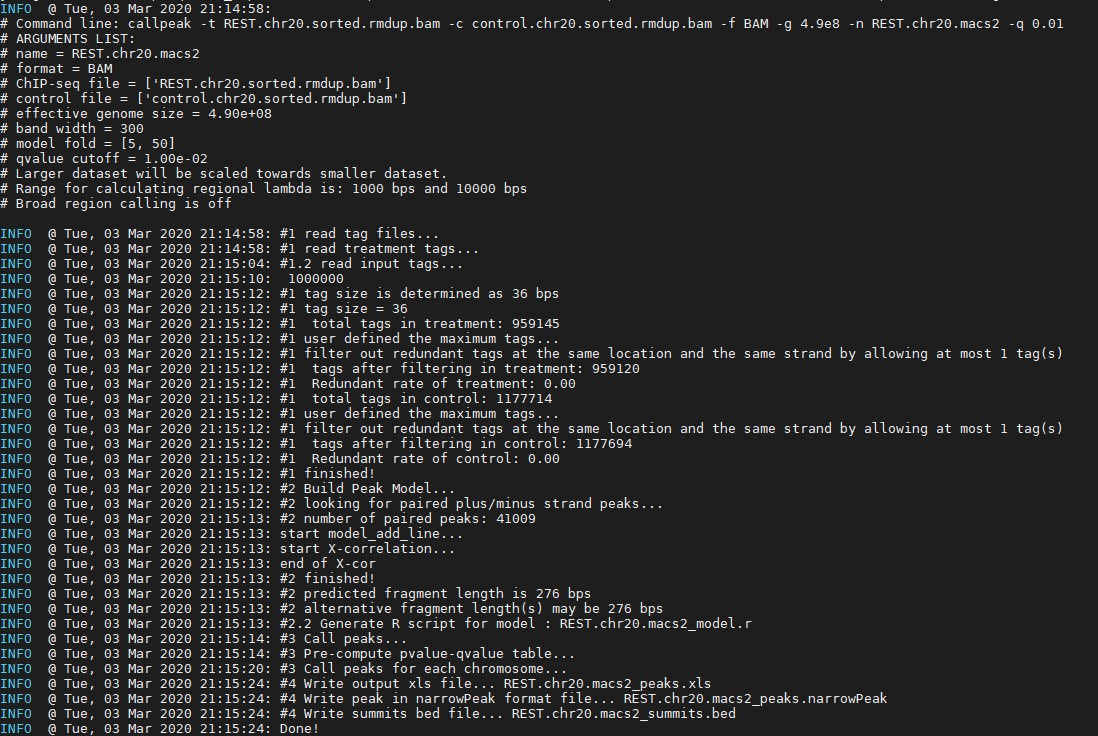
Peaks in the ChIP-seq data will be called using Model-based Analysis of ChIP-Seq (MACS2). MACS captures the influence of genome complexity to evaluate the significance of enriched ChIP regions and is one of the most popular peak callers performing well on data sets with good enrichment of transcription factors.

macs2 callpeak

macs2 callpeak -t REST.chr20.sorted.bam -c control.chr20.sorted.bam -f BAM -g 4.9e8 -n REST.chr20.macs2 -q 0.01

macs2 output

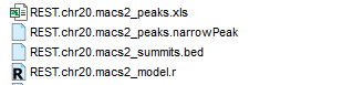
Question: please check each of the output files

5. ChIP-seq peaks visualization

The Integrative Genomics Viewer (IGV) is a high-performance visualization tool for interactive exploration of large, integrated genomic datasets. It supports a wide variety of data types, including array-based and next-generation sequence data, and genomic annotations

Install JAVA and IGV 

Directly download JAVA and IGV from official website: https://java.com/ and https://software.broadinstitute.org/software/igv/

Download the alignment and peak calling files to your locale machine 

Set reference genome hg19, load bam and peaks files (File -> Load from File)

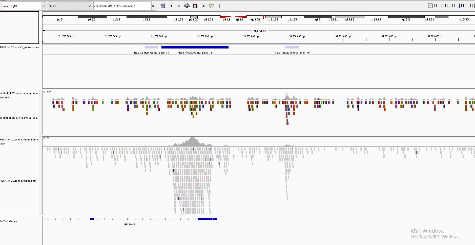
Check your results

6. Use R to analyze the ChIP-seq targets

This practice will require some programming. The basic idea of analyzing transcription targets is to overlap the ChIP-seq peaks with annotated genes. The genes with functional elements overlapped with highly significant ChIP-seq peaks would be the putative targets.

General steps

Step 0, call Dr.Tong's chip seq source codes (call the programs/function from ytong1 that I writed for you to do the analysis)

Go into a R session

>R

run R functions

options(stringsAsFactors = FALSE)

source("/home/ytong/chipseq/chipseq.fun.R")

Step 1, read in your own MACS2 result data

setwd("/home/yourfolder/your_result_folder/")

mydata<-read.table("REST.chr20.macs2_peaks.narrowPeak", sep="\t",quote="",header=FALSE)

head(mydata)

colnames(mydata)<-c("chr", "start", "end","name", "pileup", "abs_summit", "-LOG10(pvalue)","fold_enrichment", "-LOG10(qvalue)","length")

genes<-read.table("/home/reference/hg19_knowngene.promoter_1000_500.txt", sep="\t",quote="",header=TRUE)

#format your data

mydata<-data.frame(chr=paste0("chr",mydata[,1]), start=mydata[,"start"], end=mydata[,"end"], gene=NA, mydata[,4:ncol(mydata)])

genes<-data.frame(chr=genes[,1], strand=genes[,5], start=genes[,12], end=genes[,13], name=genes[,9])

head(mydata)

head(genes)

Step 2, find your targets

overlap<-overlap_bed(mydata,genes,range=1000)

overlap

Step 3, annotate your peaks

mydata[queryHits(overlap),"gene"]<-genes[subjectHits(overlap),"name"]

head(mydata)

Step 4, write result

write.csv(mydata,"REST.chr20.macs2_peaks.narrowPeak.anno.csv", quote=FALSE,row.names=FALSE)

7. Visualize the target network by cytoscape

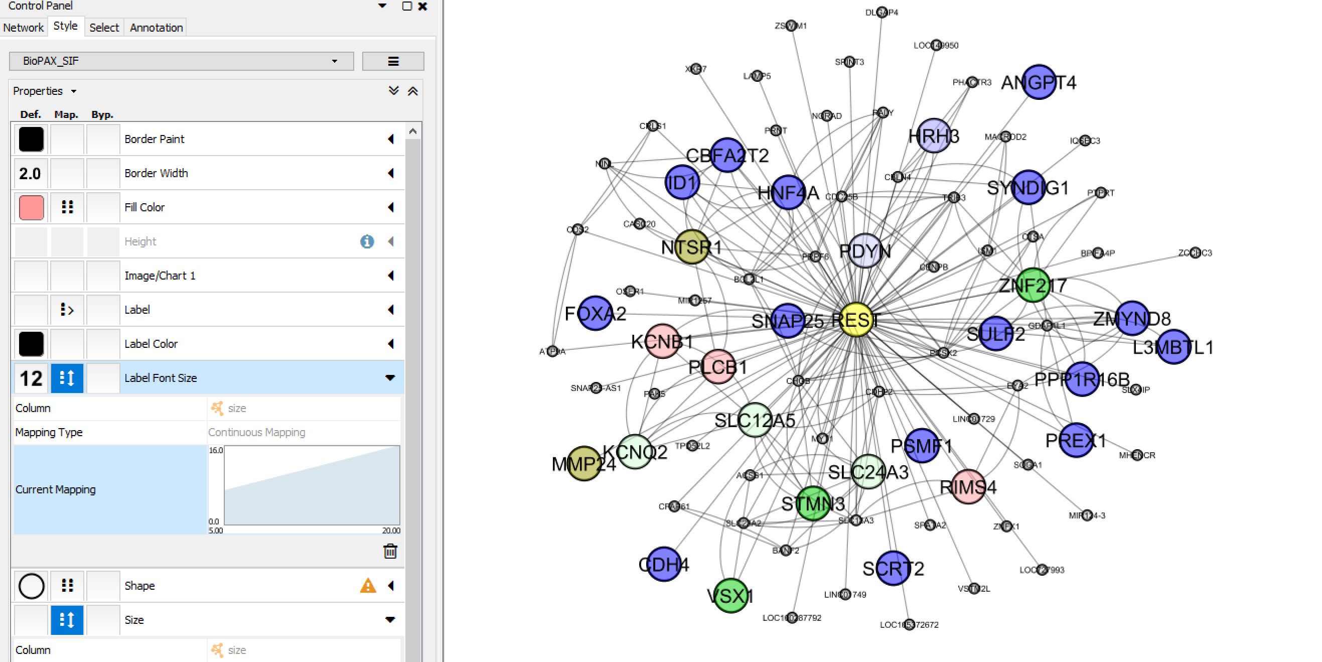
Download the annotated narrowPeak file to learn the regulation relationship between REST and its targets. Use Cytoscape to visualize the result. Cytoscape is an open source software platform for visualizing complex networks and integrating these with any type of attribute data. A lot of Apps are available for various kinds of problem domains, including bioinformatics, social network analysis, and semantic web.

Step 1, prepare the cytoscape files by the following R codes. Two files will be generated. One is network edge file: network.sif, another is network node file: network.nodes.noa

Go into a R session

>R

run R functions

options(stringsAsFactors = FALSE)

library(gage)

source("/home/ytong/chipseq/chipseq.fun.R")

setwd("/home/yourfolder/your_result_folder/")

mydata<-read.table("REST.chr20.macs2_peaks.narrowPeak.anno.csv", sep=",",quote="",header=TRUE)

target=unique(mydata$gene);target=target[!is.na(target)]

generate_network("REST",target)

This "generate network" function generates the network edge sig file with the TF "REST" in the first column and target genes in the last column. And the network node annotation files were generated by unique target genes in the first column, followed by the GO annotation of the genes, and network degree in the last column.

Step 2, visualize the TF-target network by load the files into cytoscape

You can easily download the network files generated in the last step, and load them into cytoscape

Check your results:

Tong Yin 5th-Feb 2019